Why need GNN
- utilize the structure and relationship of data (CNN cannot deal with non-Euclidean space)
- semi-supervised learning (partial labels)
How to Embed node into a feature space using convolution?
Suppose a graph \(G=\{V, E\}\), \(V\) is a set of \(N=|V|\) nodes, \(E\subseteq V\times V\) is a set of edges between nodes. There are two different groups of GNN:
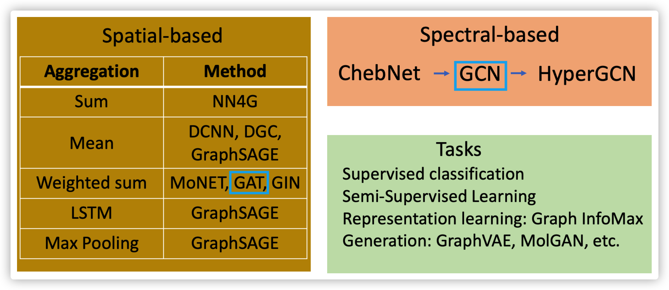
- Generalize convolution into Graph: Spatial-based Convolution
- Back into signal processing: Spectral-based Convolution
1. Spatial-based Convolution
Two important problem to be solved:
- Aggreation: how to update the next hidden sate by using neighbor's information
- Readout: how to represent graph using features from all nodes

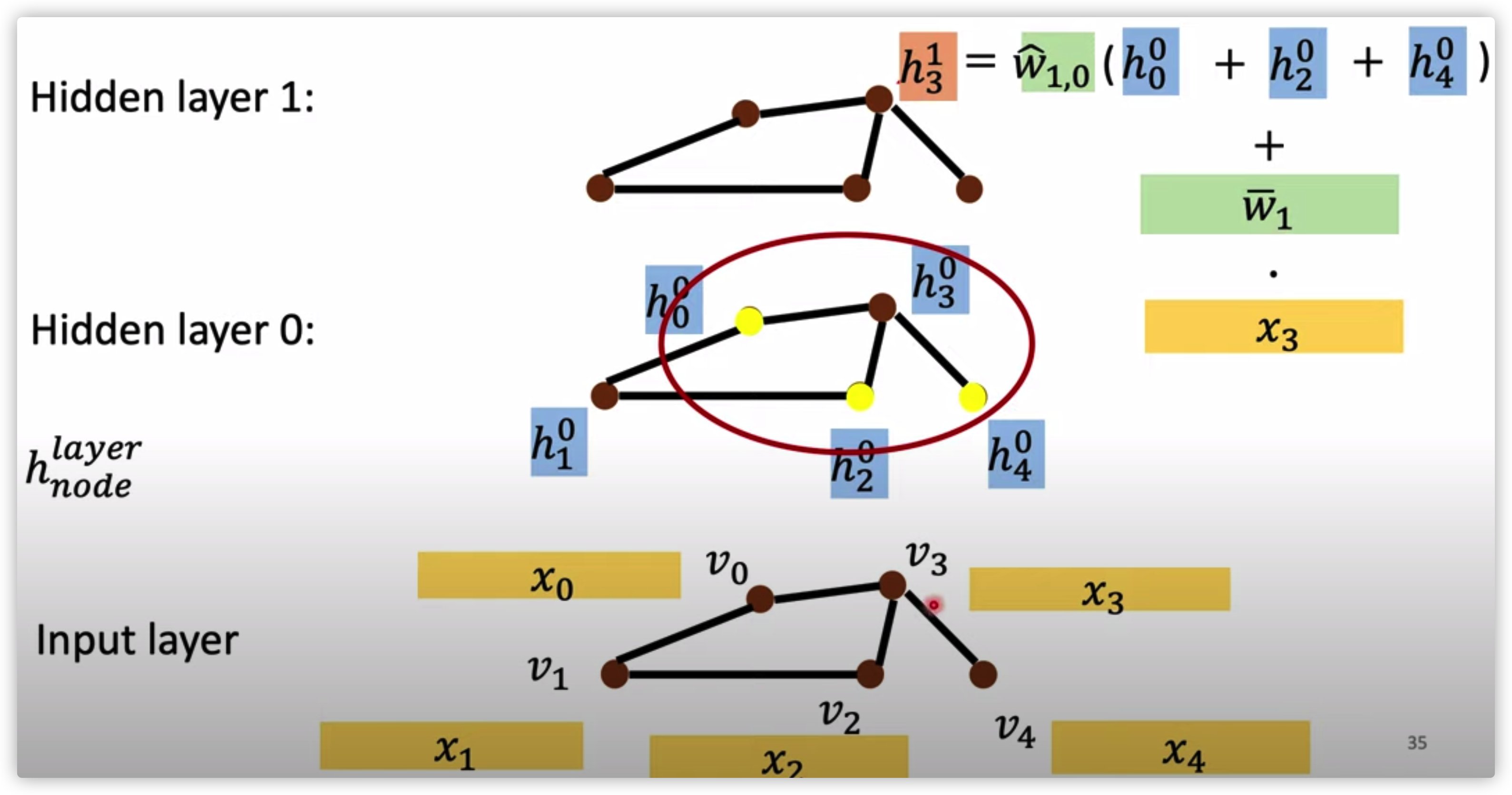
NN4G
Aggregate by sum
from input layer to \(0_{th}\) hidden layer
\(h_{n}^0=x_n \cdot w_n, n \in [1,2...,N]\)
from hidden layer \(k\) to hidden layer \(k+1\)
\(h_n^{k+1}=w_n^{k,k+1}\cdot \sum_{v\in \mathcal{N}(h_n^k)}h_v^k\)
where \(\mathcal{N}(x)\) is all neighbors of \(x\)
Readout
\(y=\sum_{k=0}^K{w_k}^T(mean(h^k)), h^k=[h_0^k,...,h_N^k]\) 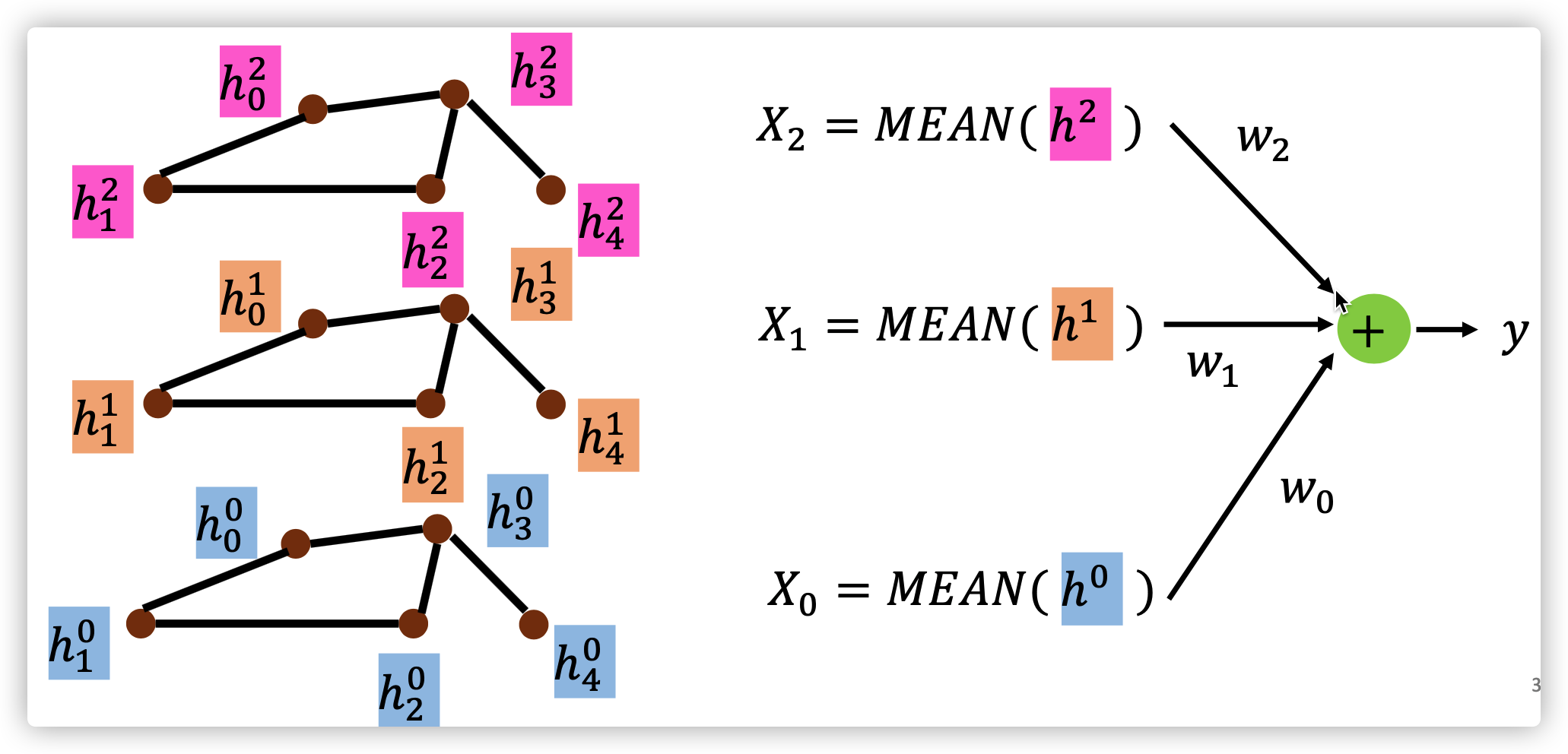
DCNN
Aggregate by mean
from input layer to \(0_{th}\) hidden layer (the same as NN4G)
\(h_{n}^0=x_n \cdot w_n, n \in [1,2...,N]\)
from hidden layer \(k\) to hidden layer \(k+1\)
\(h_n^{k+1}=w_n^{k,k+1} Mean(h_{d(n,.)=k+1}^k)\), \(d(n,.)=k+1\) is these nodes that has a distance of \(k+1\) to node \(n\)
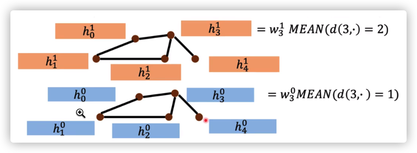
Readout
\(y_n=[h_n^0,h_n^1,...,h_n^K]^T W\)
the feature of a node \(v_1\) is 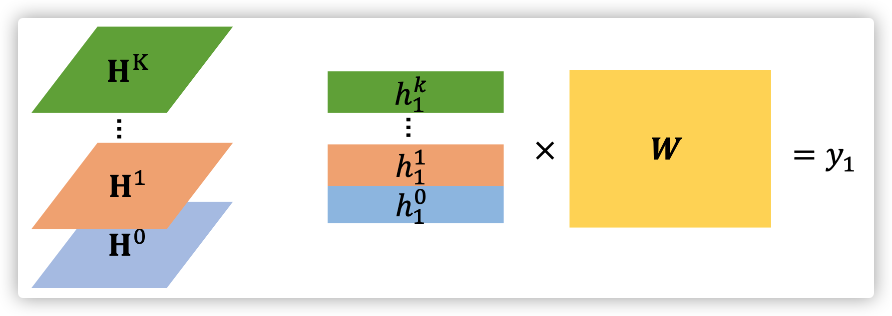
DGC
Aggregate by mean
similar to DCNN
Readout
the feature of each node is directly sum over multiple hideen sates 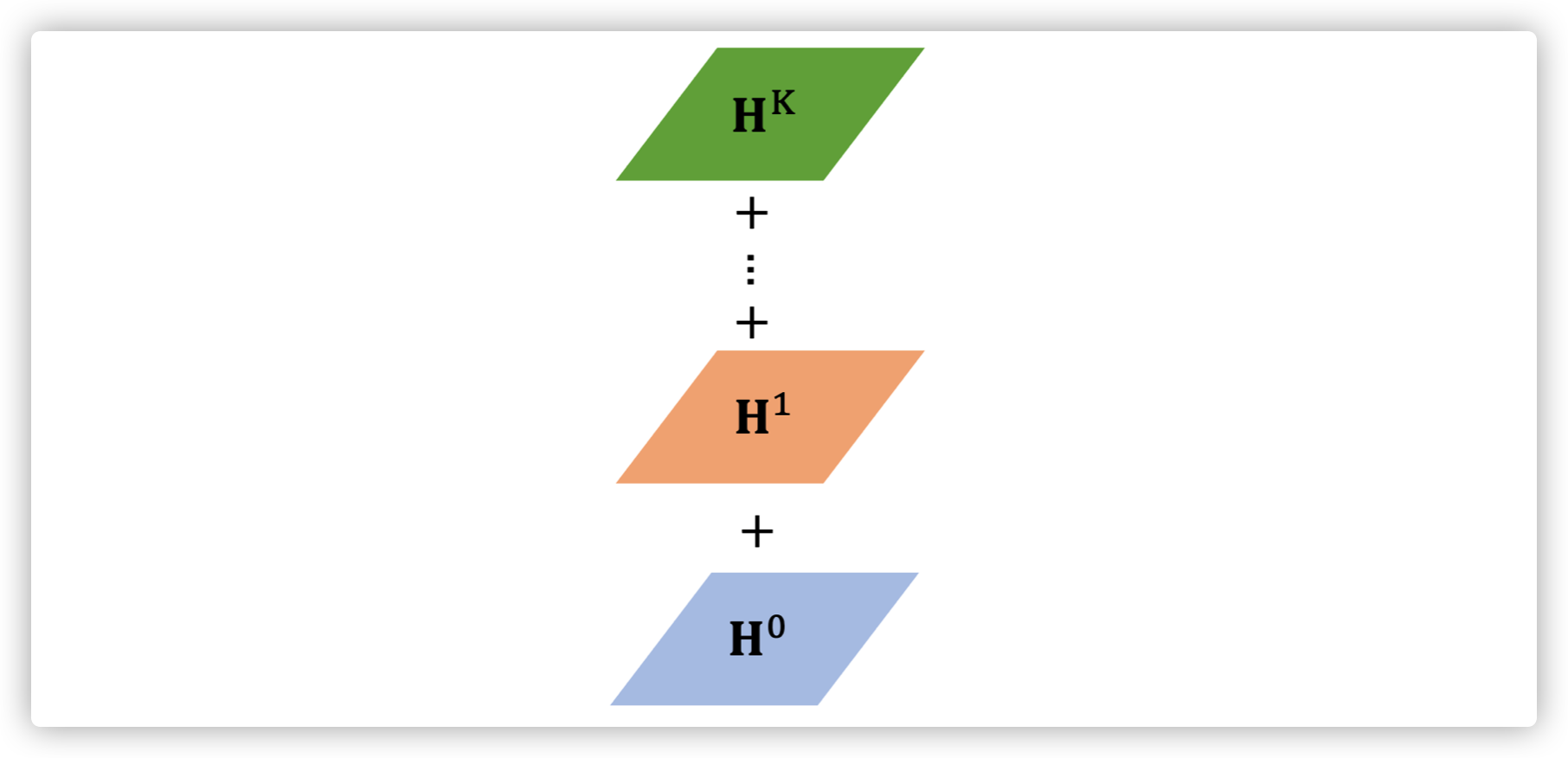
MoNET
Aggregate by weighted sum
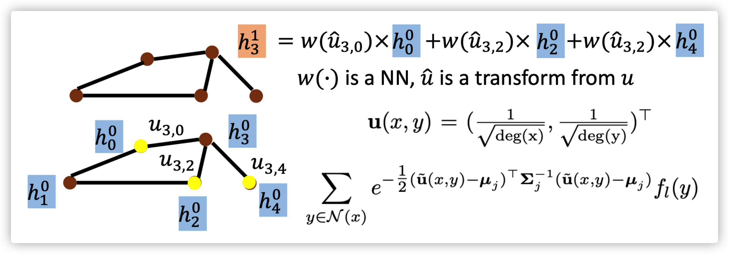

\(D_j(x)f=\sum_{y\in\mathcal{N}(x)}w_j(u(x,y))f(y),j=1,...,J\)
\((f*g)(x)-\sum_{j=1}^Jg_j D_j(x)f\)
where \(u(x,y)\) is used for measuring distance between \(x\) and \(y\), but it is a \(d\)-dementional vector. Then using a list of weight functions (kernels) \(w_{\Theta}(u)=(w_1(u),...,w_J(u))\) to extract features and aggregate feature for hidden state of next layer
Different Spatial based GNN differ in choosing on the pseudo-coordinates \(u\) and the weight functions \(w(u)\)

GraphSAGE
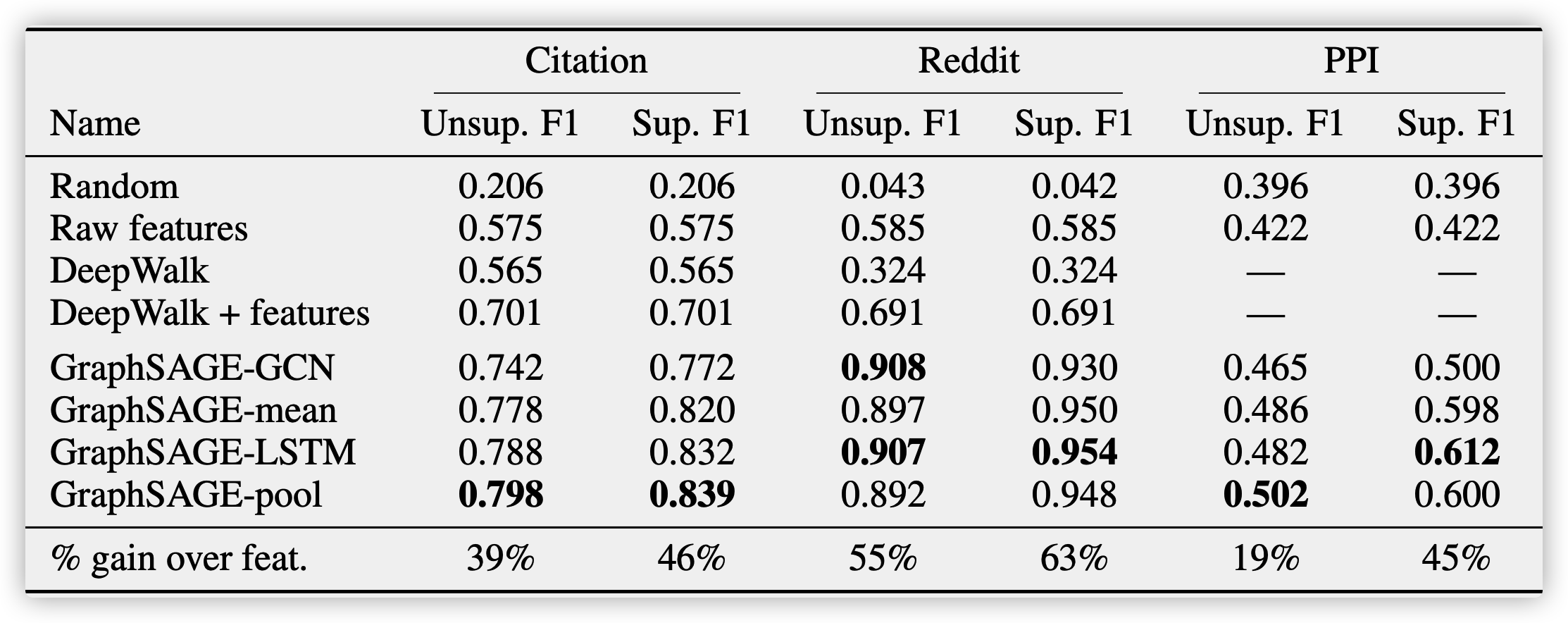
GraphSAGE is Sample and Aggregate, learning how to embed node features from neighors
Aggregate
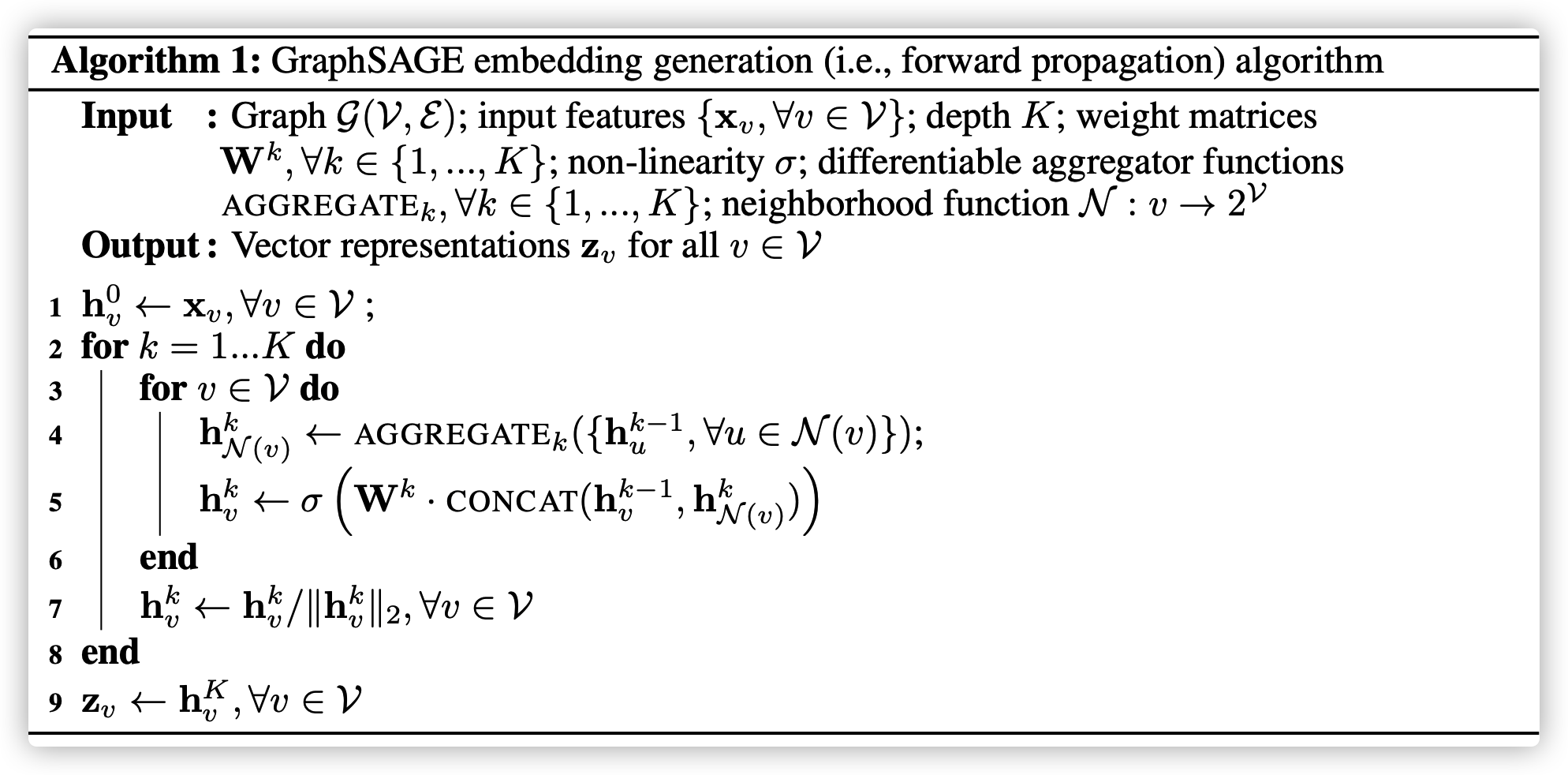
Aggregate by Mean
replace line 4 and line 5 with \(h_v^k\leftarrow \sigma(W\cdot Mean(\{h_v^{k-1}\}\cup \{h_u^{k-1}\}),u\in \mathcal{N}(v)\)
Aggregate by LSTM
applying LSTM to a random permutation of the node's neighbors
Aggregate by Pooling
\(AGGREGATE_k^{pool}=max(\{\sigma(W_{pool}h_{u}^k)+b\}), u\in\mathcal{N}(v)\)
Loss Function:
\(J_{\mathcal{G}}(z_u)=-log(\sigma(z_u^Tz_v))-Q\cdot \mathbb{E}_{v_n\sim P_n(v)}log(\sigma(-z_u^Tz_{v_n}))\)
where \(Q\) is the number of samples by negative sampling process. In supervised method, \(v\) is postive samples, \(v_n\) is negative samples; In unsupervised method, \(v\) is neighboring nodes, \(v_n\) is nodes that far away from \(u\).
GAT
In MoNet, the distance measurement \(u(i,j)\) and kernel \(w_j(u)\) is manually defined. GAT, however learn these measurements and weight functions as engergy \(e_{i,j}\).
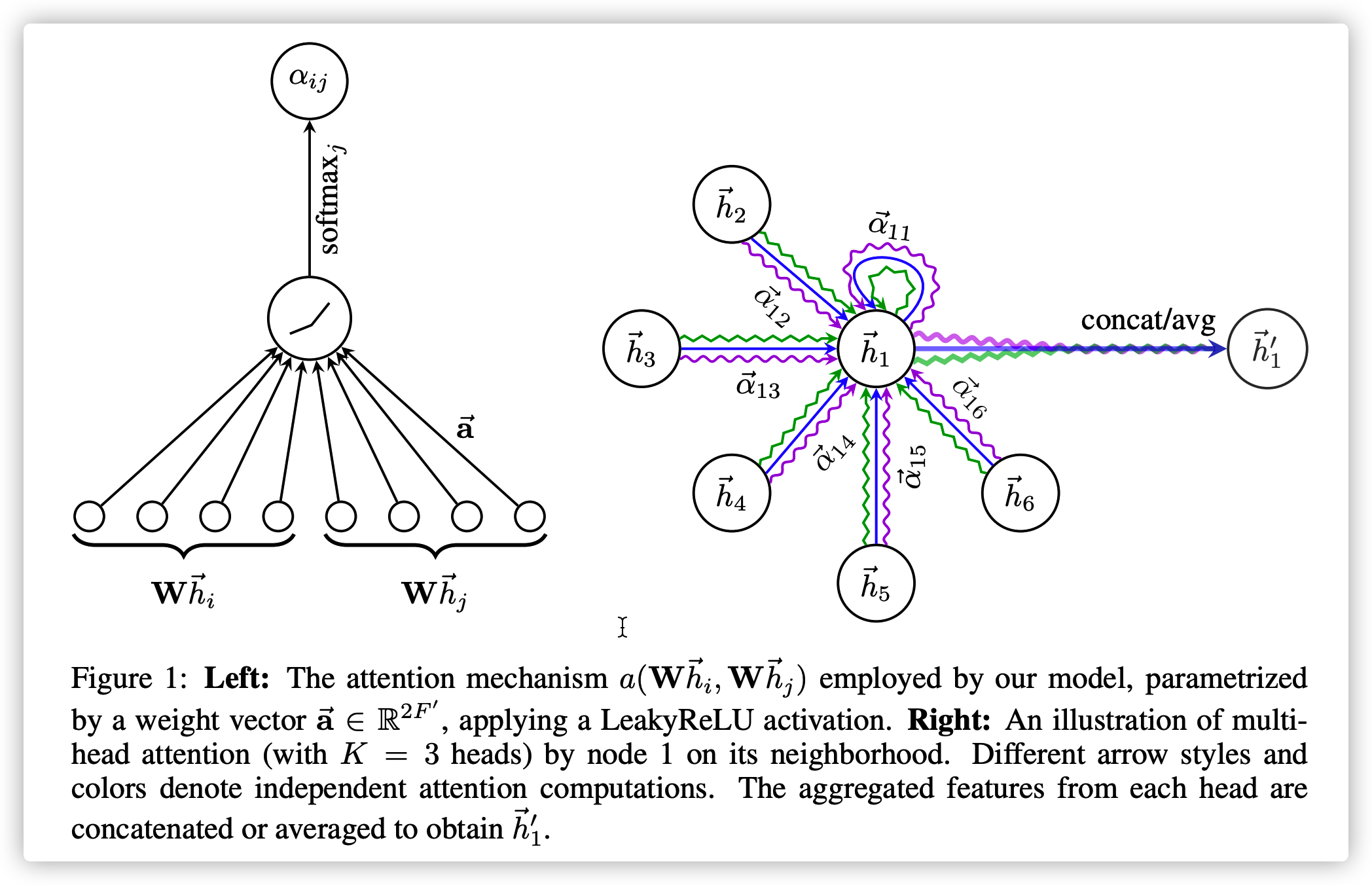
Aggregate
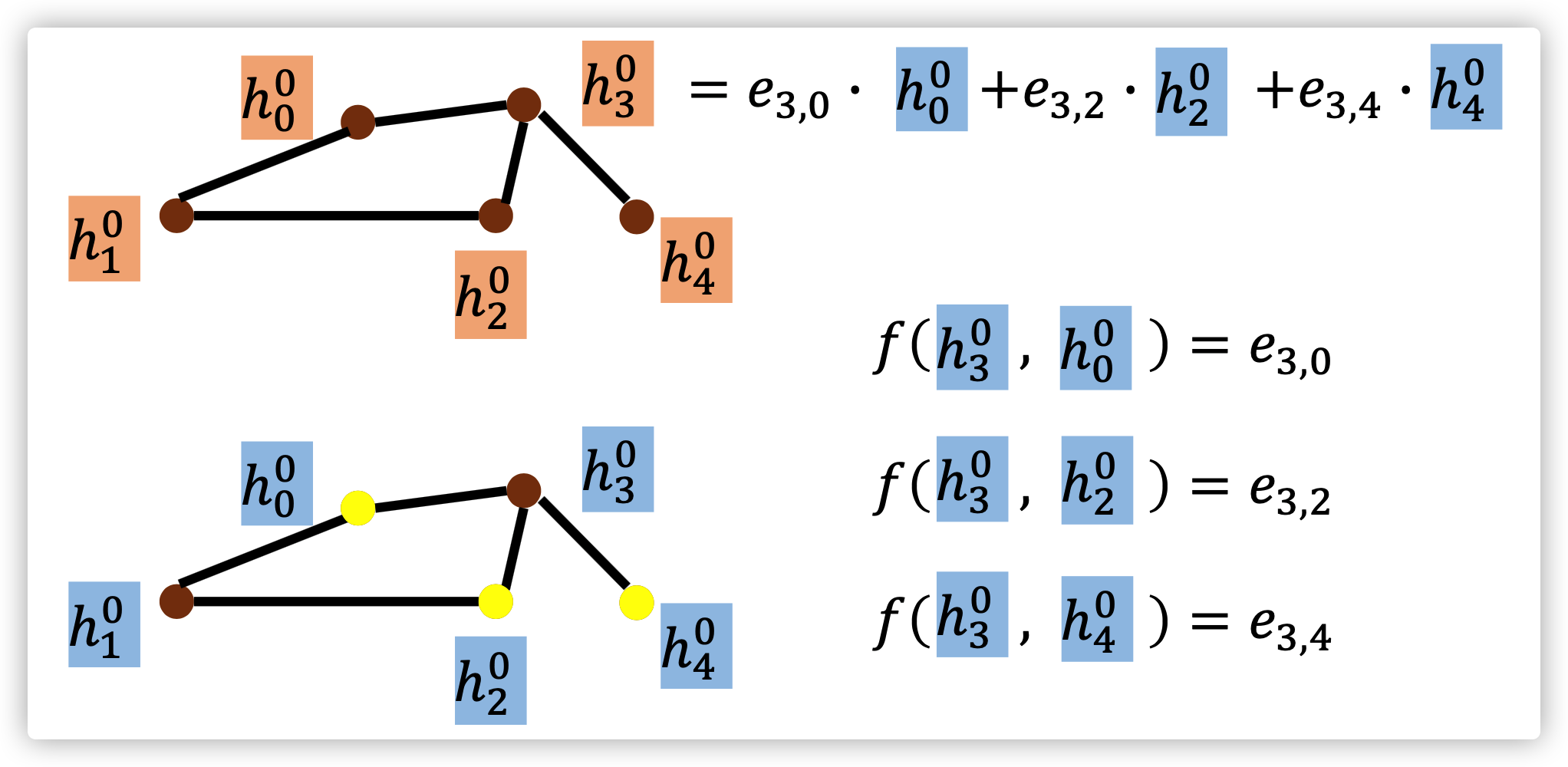
Node feature \(h=\{\vec h_1, \vec h_2,...,\vec h_N\},\vec h_i\in \mathbb{R}^F\)
Energy Calculation: \(e_{i,j}=a(W\vec h_i, W\vec h_j)\)
Attention Score over neighbors: \(a_{i,j}=\frac{exp(LeakyReLU(\vec \alpha^T [W\vec h_i || W\vec h_j]))}{\sum_{k\in\mathcal{N}(i)} exp(LeakyReLU(\vec \alpha^T [W\vec h_i || W\vec h_k]))}\)
where \(j\) is one neighbor of \(i\), \(||\) means concatenation, \(\vec \alpha \in \mathbb{R}^{2F'}\) is the parameter of the feedforward neural network
Node \(i\) is updated by \(\vec h_i' = \sigma(\sum_{j\in \mathcal{N}(i)}\alpha_{i,j}W\vec h_j)\), which is a 1-head attention. One can even use a Multi-head attention like
\(\vec h_i' = {||}_{k=1}^K \sigma(\sum_{j\in \mathcal{N}(i)}\alpha_{i,j}W^k \vec h_j)\) or \(\vec h_i' = \sigma(\frac{1}{K}\sum_{k=1}^K \sum_{j\in \mathcal{N}(i)}\alpha_{i,j}W^k \vec h_j)\)
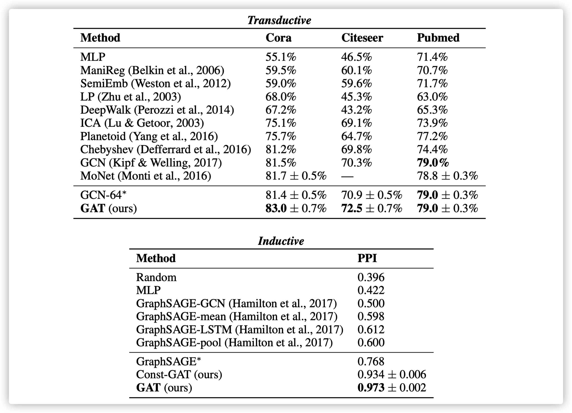
Transductive task: the feature of testing data can be used in training stage, but the label can not be observed.
Inductive task: the testing data can not be used in training stage.
GIN
A GNN can be at most as powerful as WL isomorphic test
Theoretical proofs were provided
Aggregate
\(h_v^k = MLP^{k}((1+\epsilon^k)\cdot h_v^{k-1} +\sum_{u\in \mathcal{N}(n)}h_u^{k-1})\)
- suggest using Sum instead of mean or max
- suggest using MLP instead of 1-layer

2. Spectral-based Convolution
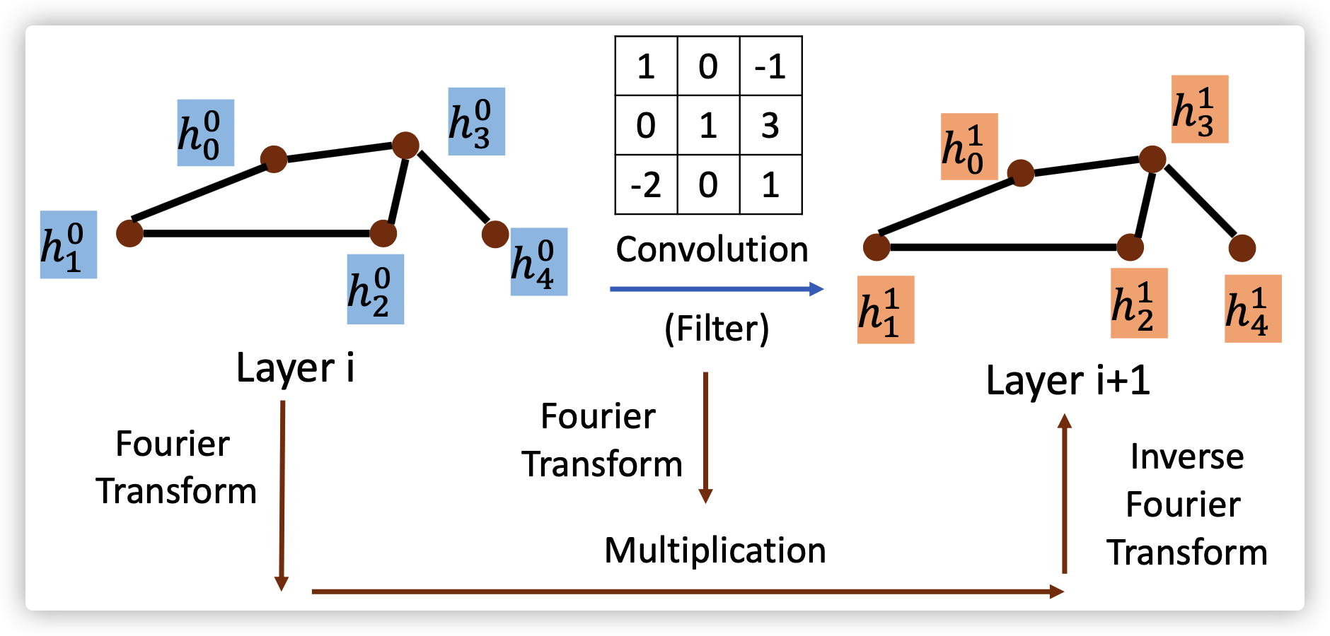
Main idea of spectral-based convolution:
transform signal from time domain into frequency domain;
using filter to process signal;
transform signal back into time domain
Different spectral-based models differ in the way of learning filter \(g_{\theta}(L)\)
Fourier Transformation
In order to understand better what's the transformation between Time Domain and Frequency Domain, thinking about the Fourier Transformation.
Time Domain
\(\vec A=\sum_i a_i \vec v_i\)
\(x(t)=\int_{-\infty}^{\infty}x(\tau)\delta(t-\tau)d\tau\)
Frequency Domain
\(\vec A=\sum_k b_k \vec u_k\)
\(x(t)=\frac{1}{2\pi}\int_{-\infty}^{\infty}X(j\omega)e^{j\omega t}d\omega\)
A signal can be represented by the weighted combination of infinite basis. The basis is \(e^{-j\omega t}\), whose weight is \(X(j\omega)\). For spectral-based Convolution GNNs, the idea is behind the designing of a list of basis and weights.

Spectral Graph Theory
the spectral graph theory will provide a way to obtaining a group of basis and their weights.
Notations
For a undirected graph \(G=(V,E),N=|V|\).
The adjacency matrix of \(G\) is \(A\in \mathbb{R}^{N\times N}\), where \(A_{i,j}=0\ if\ e_{i,j}\notin E, else\ A_{i,j}=w(i,j)\).
The degree matrix of \(G\) is \(D\in \mathbb{R}^{N\times N}\), where \(D_{i,j}=d(i)\ if\ i=j, else\ D_{i,j}=0, d(i)=\sum_j A_{i,j}\).
The signal on \(G\)(vertices) is \(f:V\rightarrow \mathbb{R}^{N}\), where \(f(i)\) denotes the signal of vertex \(i\).
Spectral Decomposition
The Laplacian Matrix of \(G\) is \(L=D-A\) (one type of Laplacian Matrix, it is positive semidefinite). Do decomposition on \(L=U\Lambda U^T\), where \(\Lambda=diag(\lambda_0,...,\lambda_{N-1})\in \mathbb{R}^{N\times N}\), \(U=[u_0,...,u_{N-1}]\in \mathbb{R}^{N\times N}\) (they are orthonormal with each other). Therefore, we found the basis \(u_n\) and its corresponding weight \(\lambda_n,n=0,...,N-1\).

Example 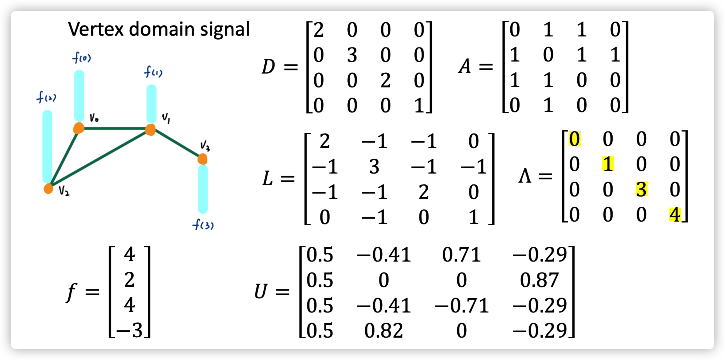
The meaning of \(Lf\) is actually represent the sum of signal (state) difference between node \(i\) and its neighbors 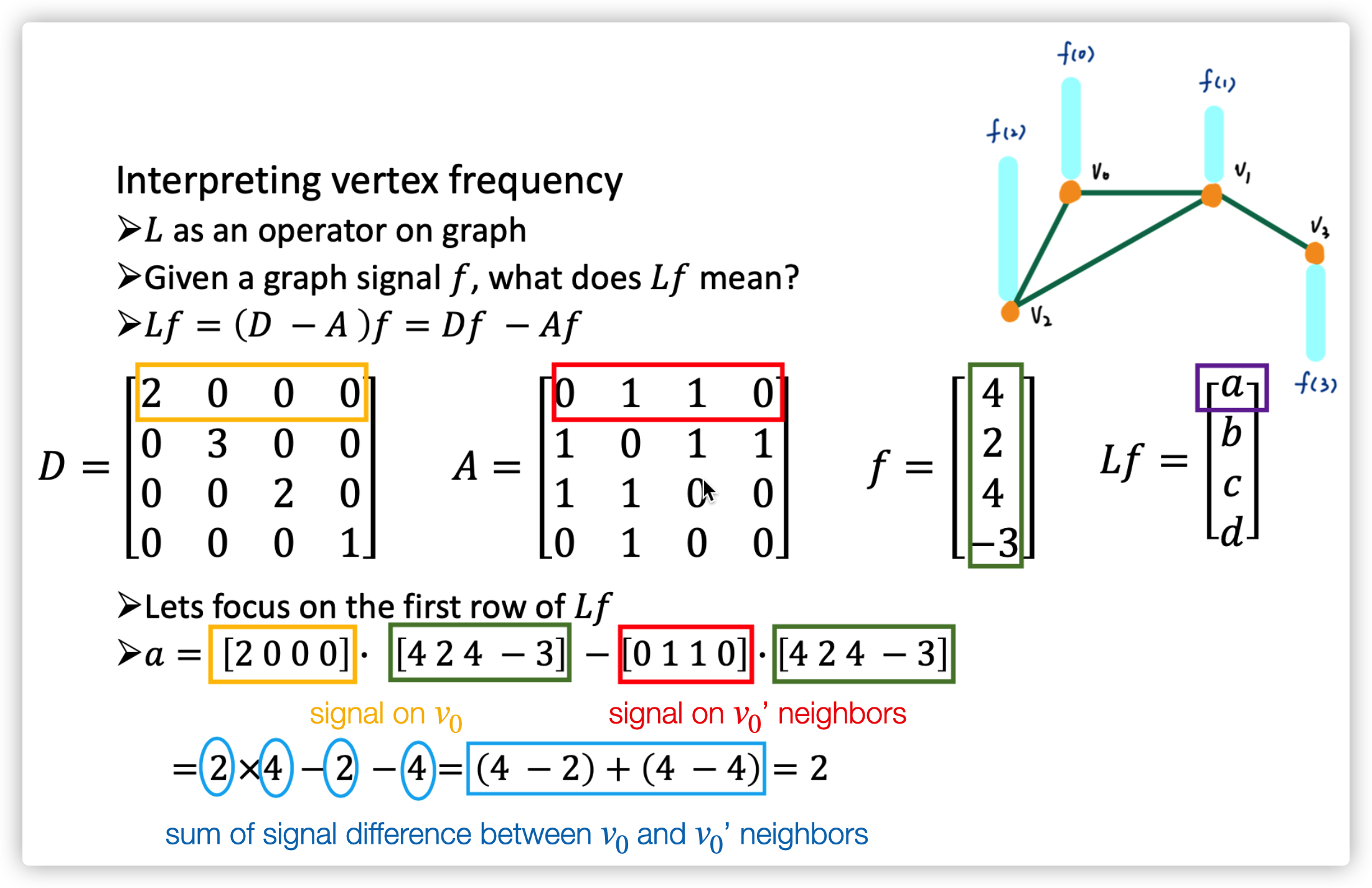
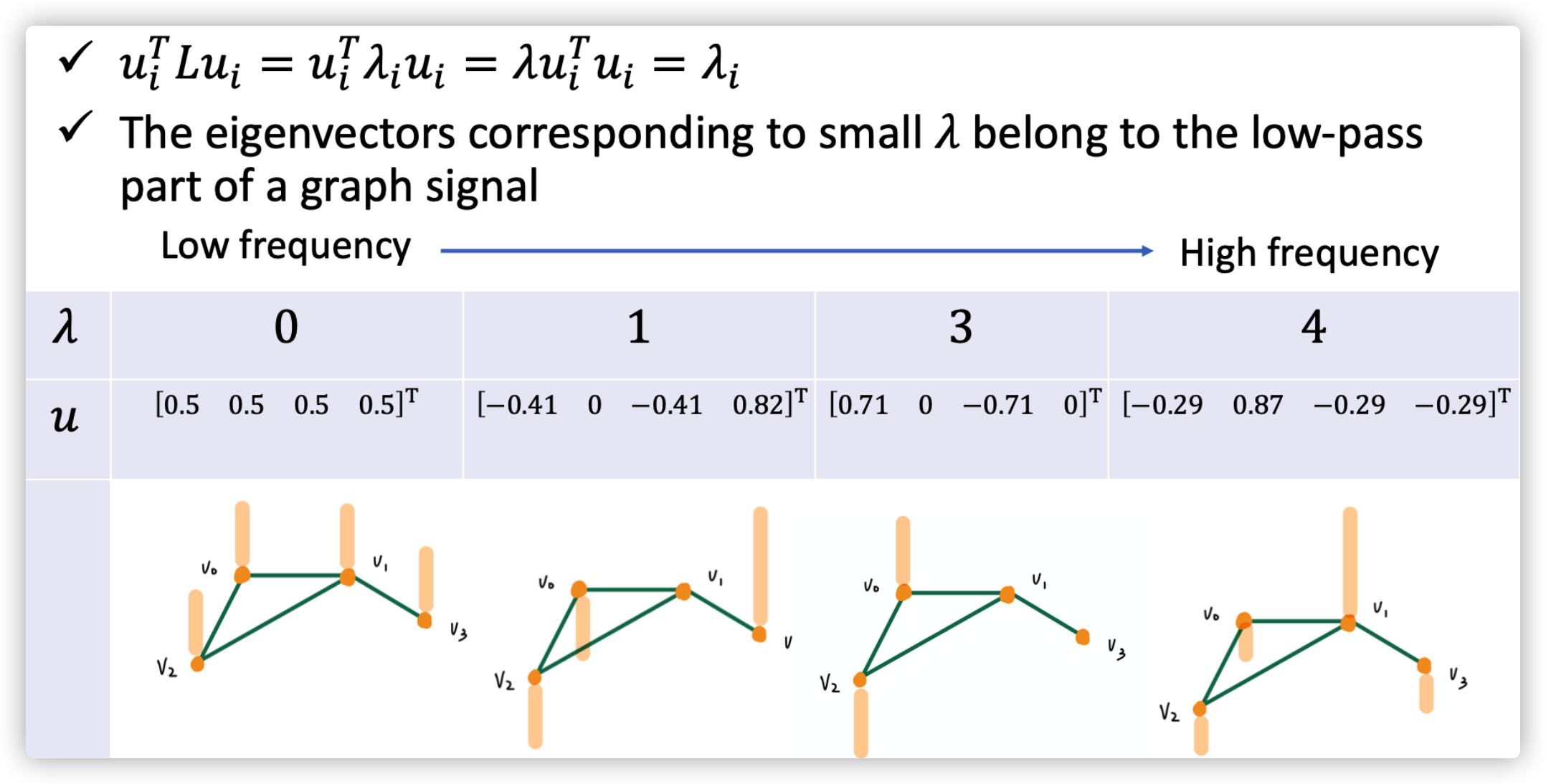
Graph Fourier Transform of signal \(\hat x=U^T x\) 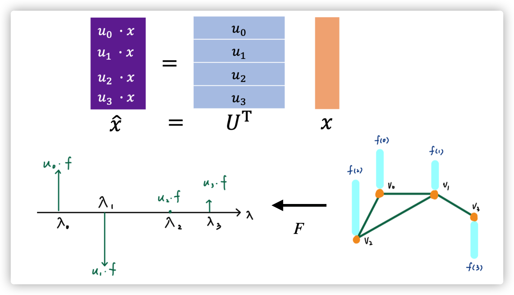
Filtering
Convolution in time domain is multiplication in frequency domain 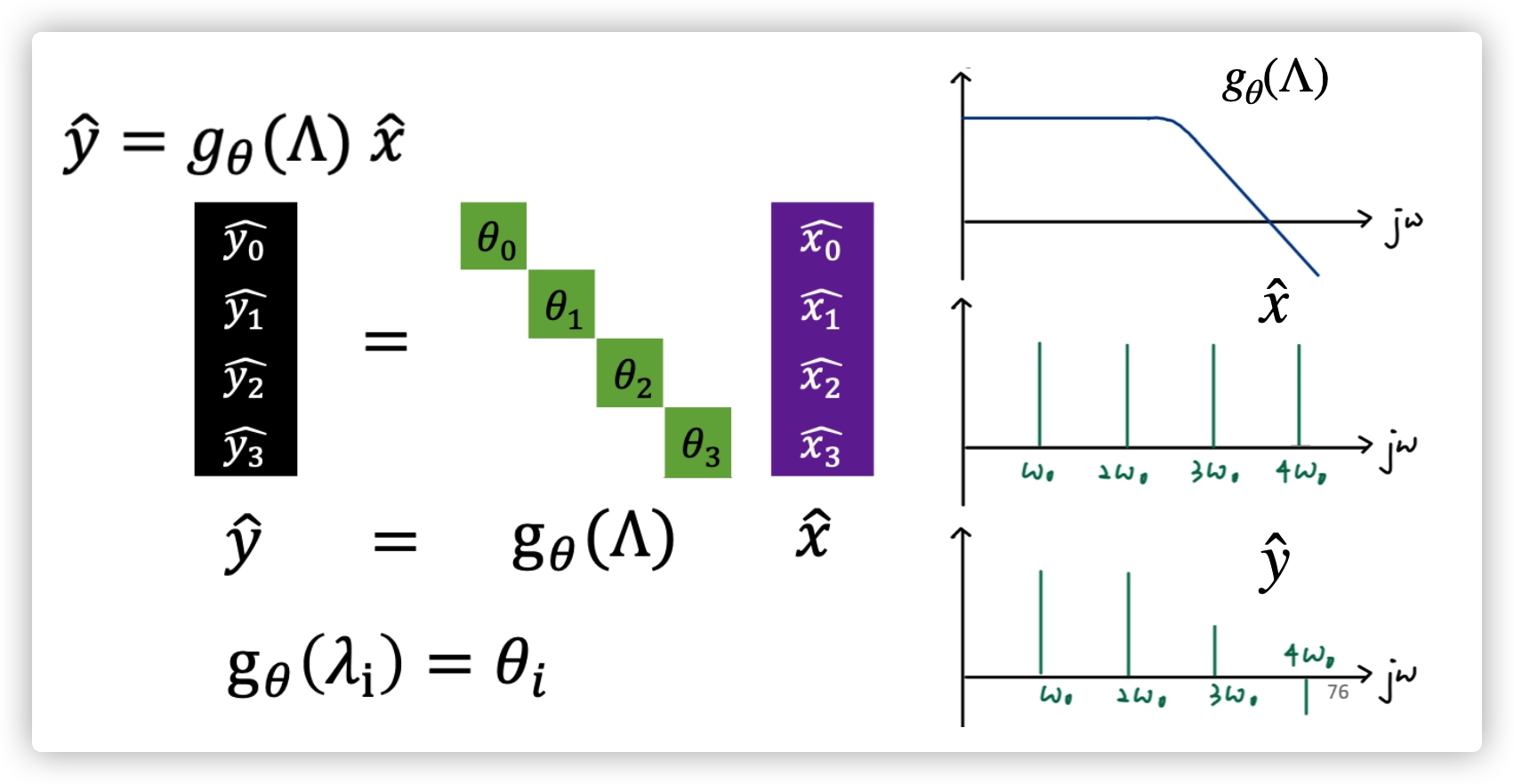
Inverse Graph Fourier Transform of signal \(x=U\hat x\) 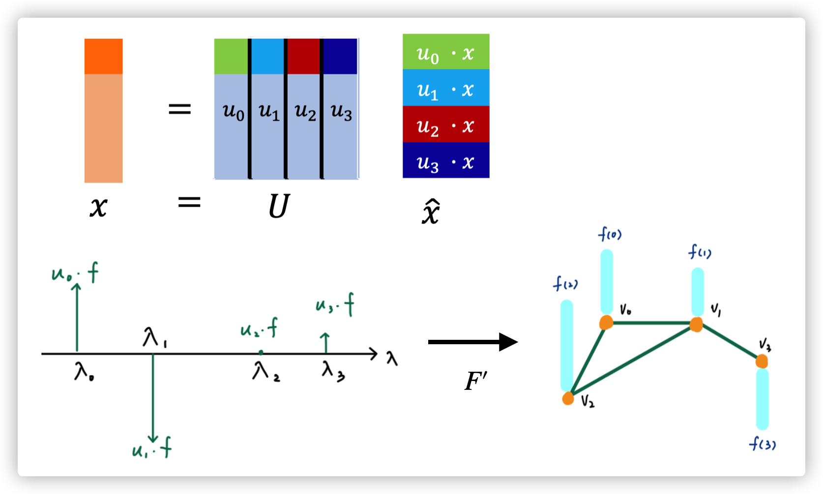
What are spectral-based GNN need to learnt?
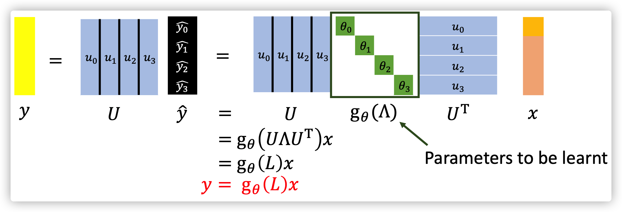 The GNN basically learnt the filter \(g_{\theta}(L)\), and this function can be any function.
For example \(g_{\theta}(L)=log(I+L)=L-\frac{L^2}{2}+\frac{L^3}{3}..., L=D-A\).
Two problem will happen if we use this function \(log(I+L)\)
- The size of parameters is growing up with \(O(N)\), \(N=|V|\) is dimention of \(\theta\). Because the decomposition of \(L\) must produce \(N\) eigenvectors (bases)
- The signal \(y\) is not localized (over smoothing). Because when \(k\) (of \(L^{k}\)) becomes bigger, signal of all other nodes will be aggregated in current node. finally, the output of different nodes will be the same. (\(K\) should be resonably small)
- The decomposition of \(L\) is time-costing \(O(N^2)\)
When \(g_{\theta}(L)=L\), each node will just consider aggregate the information from their neighbors. When \(g_{\theta}(L)=L^2\), each node will consider all nodes that has a distance (within 2) from this node. \(x=[f(0),f(1),f(2),f(3)]\) 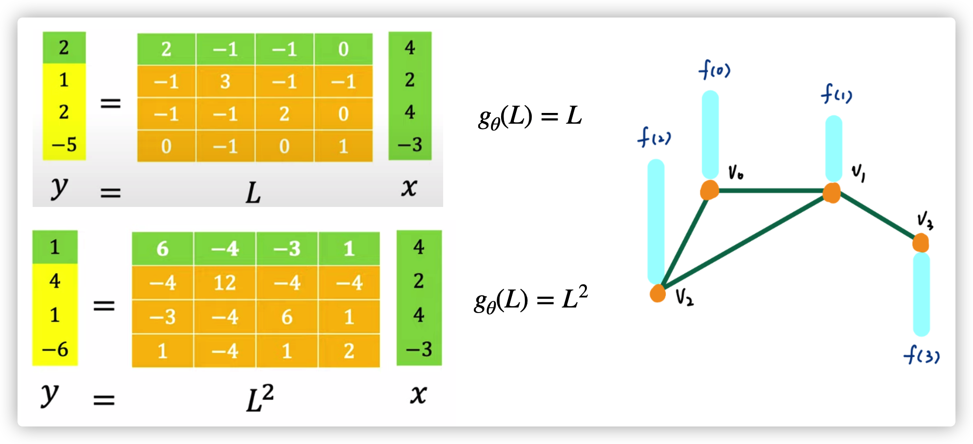
Therefore all those spectral-based GNN use different strategy to overcome the difficulty of learning \(g_{\theta}(L)\)
ChebNet
ChebNet use polynomial to parametrize \(g_{\theta}(L)\) and prevent the decomposition of \(L\) (explicitly calculate eigenvectors). The localization is managed by \(K\) (K-hop neighbors).
\(g_{\theta}(L)=\sum_{k=1}^K \theta_k L^k\)
\(g_{\theta}(\Lambda)=\sum_{k=1}^K \theta_k \Lambda^k\)
\(y=Ug_{\theta}(\Lambda)U^Tx=\sum_{k=1}^K \theta_k L^kx=U(\sum_{k=1}^K \theta_k \Lambda^k)U^Tx\)
Therefore, the size of parameter is \(K\), and the localization is fixed by \(K\). But the calculate \(L^k\) and obtaining eigenvectors \(U\) need time complexity of \(O(N^2)\)
Therefore Chebyshev poluyomial is used to calculate \(\Lambda^k\) in a recursive way and also prohibit the calculation of eigenvectors \(U\).
\(T_0(\tilde \Lambda)=I, T_1(\tilde \Lambda)=\tilde{\Lambda}, T_l(\tilde \Lambda)=2\tilde \Lambda\ T_{k-1}(\tilde \Lambda)-T_{k-2}(\tilde \Lambda)\), where \(\tilde \Lambda=\frac{2\Lambda}{\lambda_{max}}-I, \tilde \lambda\in[-1,1]\)
\(g_{\theta}(\Lambda)=\sum_{k=1}^K \theta_k \Lambda^k\rightarrow g_{\theta'}(\Lambda)=\sum_{k=1}^K \theta_k' T_k(\tilde{\Lambda})\)
Therefore the final signal \(y\) can be efficiently computed, \(y=g_{\theta'}(\tilde{L})x=\sum_{k=1}^K \theta_k' T_k(\tilde{L})x\) 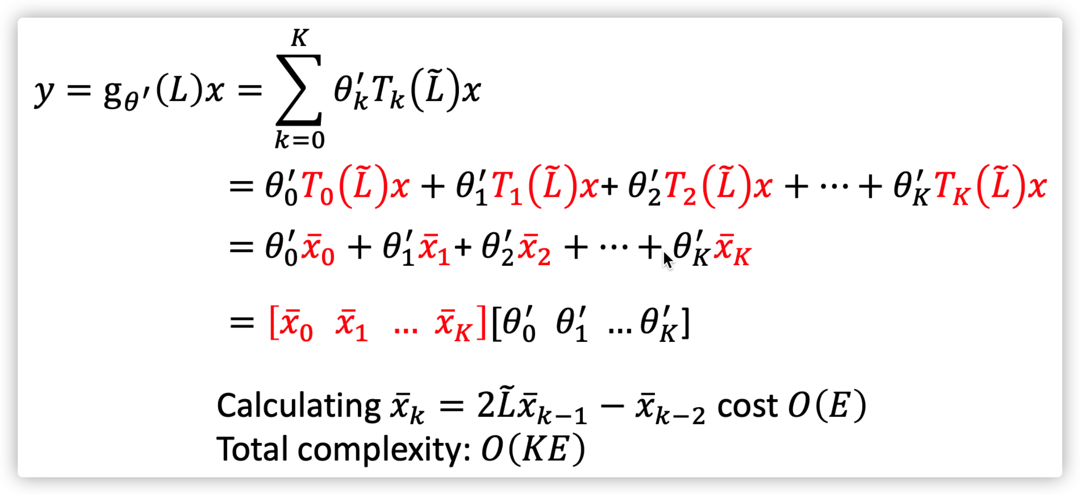 ChebNet
GCN
The designing of \(g_{\theta}(L)\)
\(y=g_{\theta'}(L)x\approx \sum_{k=0}^K\theta_k' T_k(\tilde{L})x, K=1\)
\(y=g_{\theta'}(L)x\approx\theta_0'x+\theta_1'\tilde{L}x,\ \ \ \ \tilde{L}=\frac{2L}{\lambda_{max}}-I\)
\(=\theta_0'x+\theta_1'(\frac{2L}{\lambda_{max}}-I)x,\ \ \ \ \lambda_{max}\approx 2\)
\(=\theta_0'x+\theta_1'(L-I)x,\ \ \ \ L=I-D^{-\frac{1}{2}}AD^{-\frac{1}{2}}\)
\(=\theta_0'x-\theta_1'(D^{-\frac{1}{2}}AD^{-\frac{1}{2}})x,\ \ \ \ \theta=\theta_0'=-\theta_1'\)
\(=\theta(I+D^{-\frac{1}{2}}AD^{-\frac{1}{2}})x\)
Use the renomalization trick: \(I+D^{-\frac{1}{2}}AD^{-\frac{1}{2}}\rightarrow \tilde{D}^{-\frac{1}{2}}\tilde{A}\tilde{D}^{-\frac{1}{2}}\), where \(\tilde{A}=A+I\), and \(\tilde{D}_{ii}=\sum_j \tilde{A}_{i,j}\)
Therefore, the classic GCN use \(y\approx \theta(\tilde{D}^{-\frac{1}{2}}\tilde{A}\tilde{D}^{-\frac{1}{2}})x\), why GCN use \(\tilde{D}^{-\frac1{2}}\), because it can reduce the information from neighbors according to the degree of node. Node with a few neighbors will get more information from its neighbors, while node with many neighbors should get less information from its neighbors.
The updating function of layer \(l+1\) is \(H^{(l+1)}=\sigma(\tilde{D}^{-\frac{1}{2}}\tilde{A}\tilde{D}^{-\frac{1}{2}}H^{(l)}W^{(l)})\)
An example of 2 layer GCN is
\(Z=f(X,\tilde{A})=softmax(\tilde{A}\ ReLU(\tilde{A}X\ W^{(0)})\ W^{(1)}), \tilde{A}=\tilde{D}^{-\frac{1}{2}}\tilde{A}\tilde{D}^{-\frac{1}{2}}\)
HyperGCN
reference paper 2019 NeurIPS deals with the network of co-author, co-citation. The main idea is simplifying the hypergraph into a simple graph that can be processed by GNN.
Hypergraph 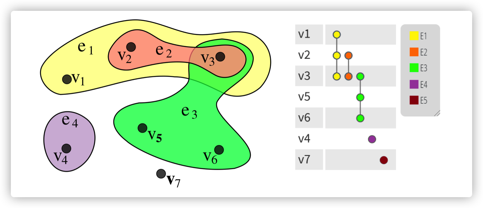
Graph Convolution on a hypernode \(v\) using HyperGCN, where
\(\tau\) is the number of epoch
\(h_v^{\tau+1}\) is the hidden state in epoch \(\tau+1\)
\(\mathcal{N}(v)\) is neighbors of node \(v\)
\([\bar A_s^{(\tau)}]_{u,v}\) is the normalized weight between node \(v\) and \(u\)

Differences between Spatial-based GNN and Spectral-based GNN
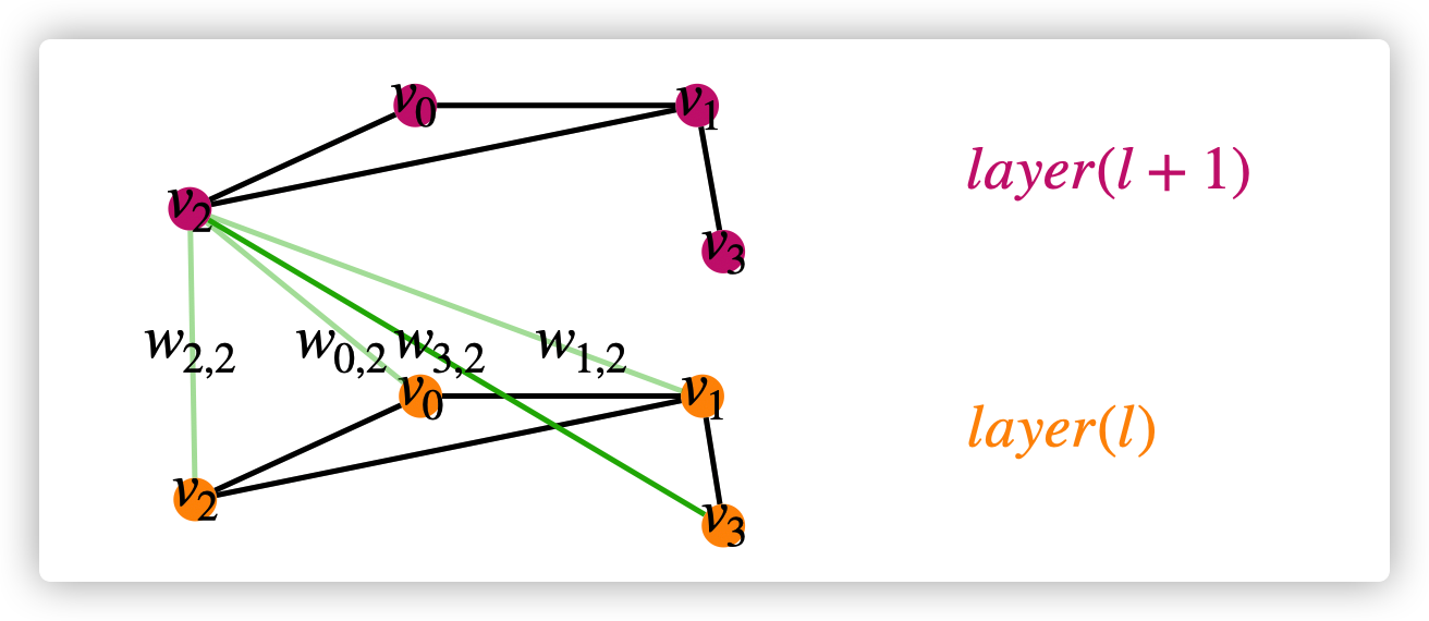
- Spectral-based GNN can not assign different weights for neighbors in different hop, GAT (spatial-based GNN) solved this problem. For example, \(w_{0,2},w_{1,2},w_{2,2}\) are hop-1 neighbors of \(v_2\), while \(w_{3,2}\) is is hop-2 neighbor of \(v_2\). In spectral-based GNN, \(w_{0,2}=w_{1,2}=w_{2,2}\neq w_{3,2}\); in GAT, \(w_{0,2}\neq w_{1,2}\neq w_{2,2}\neq w_{3,2}\)
Python implementation of GNN
Dataset
- CORA: citation network. 2.7k nodes and 5.4k links
- TU-MUTAG: 188 molecules with 18 nodes on average
Summarization
